Prev: Chi Square test | Next: Write your own ANOVA function

One way ANOVA¶

What is ANOVA¶

The ANOVA name (from 'ANalysis Of VAriance') stands for a family of statistical controls that test for statistical significance between sample means by examining the sample variances.
When we simply refer to 'ANOVA', we usually mean the 'one way' ANOVA which is a test for exploring the impact of one single factor on three or more groups (but two groups would also do, as we explain below).

Examples of use:

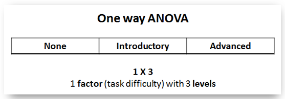
In educational research: Suppose you want to investigate the impact of an instructional method when tasks of varied difficulty are assigned to students. You randomly distribute your students to three groups and implement the instructional method differently for each group: group-1: no tasks at all, group-2: introductory level tasks, group-3: advanced level tasks. Later you run a post-test questionnaire to record students' learning performance. You apply a one way ANOVA to statistically compare the post-test performance in the three student groups. In your design you have: one factor (task difficulty) with three levels (none, introductory, advanced).

What to know about ANOVA¶

Apply one way ANOVA when you have data from three or more independent samples and no pre-test data (that is, baseline data before the intervention). In this latter case it is more appropriate to apply ANCOVA ('analysis of covariance' with baseline measurement as covariate).
Apply ANOVA even for two groups instead of a t-test. ANOVA is a more powerful test and will be more sensitive in identifying a statistical significance if one really exists.
ANOVA is based on F distribution; thus ANOVA controls return the F statistic and the p probability. A thorough explanation of how ANOVA algorithm computes the F statistic is provided in the next section.
Applying solely ANOVA is not adequate. This is because:
- ANOVA tells us about 'main interactions', that is, whether there is a statistically significant difference between the means of the groups, but does NOT tell which exactly pair (or pairs) of groups causes this significance.
- Therefore, after applying ANOVA, a number of specialized t-tests (usually Tukey or Bonferoni) have to be also applied (this is discussed at the end of this section).

An ANOVA scenario¶

We continue our 'background music' scenario: so far in our experimentation we have been using as background music mainly 'soft' tunes which supposedly help students relax and concentrate on their study. However, we wonder what would have happened in case we used some more vivid ('modern') tunes in the background. We suspect this would act as a distractor but nevertheless we would like to have some concrete data.
So, we design the following experiment:
- IV: Background music (three conditions: 1) no b.m., 2) soft tune, 3) modern tune
- DV: Learning performance as measured by some reliable and validated test (continuous variable, scale 0-100)
- Population: students of specific age and background studying in a multimedia elearning environment
- Research Design: Three groups post-test only design
- Groups:
  - Control (C-group): N0=40 students (randomly selected) studying without background music
  - Treatment1 (T1-group): N1=42 students (randomly selected) studying with soft background music
  - Treatment2 (T2-group): N2=43 students (randomly selected) studying with modern background music
- Null hypothesis H₀ = "Students studying with background music (either soft or modern) will perform the same in an appropriate knowledge test with students studing without background music" (non-directional)

Read and clean data¶

Read data from researchdata.xlsx file ('anova' spreadsheet) and remove non existing entries

import pandas as pd 
import scipy.stats as stats

data = pd.read_excel('../../data/researchdata.xlsx', sheetname="anova")
data.head()
data.tail()

dC = data.Control.dropna()
dT1 = data.Treatment1.dropna()
dT2 = data.Treatment2.dropna()

Sample descriptive statistics¶

print('Control group\n')
print(dC.describe())
print('\nTreatment-1 group\n')
print(dT1.describe())
print('\nTreatment-2 group\n')
print(dT2.describe())

Control group

count    40.000000
mean     69.500000
std      10.919284
min      47.000000
25%      62.000000
50%      69.500000
75%      77.000000
max      92.000000
Name: Control, dtype: float64

Treatment-1 group

count    42.000000
mean     75.428571
std      10.551021
min      54.000000
25%      69.000000
50%      74.000000
75%      84.000000
max      94.000000
Name: Treatment1, dtype: float64

Treatment-2 group

count    43.000000
mean     68.790698
std      11.306463
min      42.000000
25%      62.000000
50%      67.000000
75%      77.000000
max      92.000000
Name: Treatment2, dtype: float64

Apply one way ANOVA¶

Test for normality/variance criteria¶

The assumptions for implementing one way ANOVA include (as in independent sample t-test):
- The normality criterion: each group compared should come from a population following the normal distribution.
- The variance criterion (or 'homogeneity of variances'): samples should come from populations with the same variance.
- Independent samples: performance (the dependent variable) in each sample should not be affected by the conditions in other samples.

# Shapiro-Wilk normality test 
stats.shapiro(dC), stats.shapiro(dT1), stats.shapiro(dT2)

((0.9695044159889221, 0.3470972180366516),
 (0.9589287638664246, 0.13518860936164856),
 (0.9781549572944641, 0.5761716961860657))

All p values are greater than threshold a = 0.05, therefore we "fail to reject" the null hypothesis (conclusion: samples come from populations that follow normal distribution).

# Levene variance test  
stats.levene(dC, dT1, dT2)

LeveneResult(statistic=0.054610924231632968, pvalue=0.9468766068380543)

p value is greater than threshold a = 0.05, therefore we "fail to reject" the null hypothesis (conclusion: samples come from populations with the same variance)

Apply one way ANOVA by calling the f_oneway() method¶

F, p = stats.f_oneway(dC, dT1, dT2)
print('F statistic = {:5.3f} and probability p = {:5.3f}'.format(F, p))

F statistic = 4.668 and probability p = 0.011

Interpretation of results¶

As p < a (0.05) we state that we have a main interaction effect. This simply means that amongst group comparison identifies statistically significant differences. However, this result does not identify the sample pair (or pairs) which cause this significance.
So, when ANOVA reports 'interaction effect' we need to further identify the group pairs by applying pair-wise controls. Although these controls could be done by implementing ordinary t-test (as demonstrated below) this is not the right approach.

# apply ttest_indep()
t, p = stats.ttest_ind(dC, dT1)
print('Control vs T1:', t, p)

t, p = stats.ttest_ind(dC, dT2)
print('Control vs T2:', t, p)

t, p = stats.ttest_ind(dT1, dT2)
print('T1 vs T2:', t, p)

Control vs T1: -2.50041403265 0.0144483070958
Control vs T2: 0.290324951396 0.772309638885
T1 vs T2: 2.79684526009 0.00641163398569

Apply Tukey's test¶

Why a special test here?¶

The simple answer is that compared to multiple Student's t-tests the Tukey's test makes a correction necessary in this case (when multipe group comparisons are implemented) and returns a much more accurate estimation of significance.
This correction is relevant to minimizing the chances for Type I error in hypothesis testing, which is: "erroneously rejecting the null hypothesis which is true".
You can read more about Tukey'test@wikipedia and also about Type I and type II errors"@wikipedia
Note that the test is also known as "Tukey's HSD (honest significant difference) test". This explains why the relevant method is named as "tukeyhsd()" (see code example below)

In practice¶

Scipy does not currently support Tukey's test but a more recent and advanced statistical package ("statsmodels") does.
So, to implement Tukey's test we need to:
- (a) Import from statsmodels.stats the multicomp module
- (b) Call the MultiComparison class constructor and pass as arguments:
  - an array of data ('Score' in the example code below)
  - an array of labels ('Group' in the example code below)
- (c) Finally, call method tukeyhsd() of the Multicomparison object and print the outcome.
Read more about MultiComparison class@statsmodel documentation

import pandas as pd
import statsmodels.stats.multicomp as ml

# Note that data in sheet have been preformatted in Group and Score columns 
dtuk = pd.read_excel('../../data/researchdata.xlsx', sheetname="multicomp")
print(dtuk.head(),'\n')

mcobj = ml.MultiComparison(dtuk.Score, dtuk.Group)
out = mcobj.tukeyhsd(0.05) 

print(out)

  Group  Score
0     C     62
1     C     67
2     C     72
3     C     77
4     C     72 

Multiple Comparison of Means - Tukey HSD,FWER=0.05
==============================================
group1 group2 meandiff  lower    upper  reject
----------------------------------------------
  C      T1    5.9286   0.197   11.6601  True 
  C      T2   -0.7093  -6.4082   4.9896 False 
  T1     T2   -6.6379  -12.2661 -1.0097  True 
----------------------------------------------

Interpretation of results¶

tukeyhsd() method returned a table with pair-wise statistics. Note that in the 'reject' column for C-T1 and T1-T2 pairs a 'True' appears while the entry for the C-T2 pair is 'False'
These boolean values refer to whether we should reject the null hypothesis that the means of the tested pair are statistically similar (non-significant differences). Thus, we reject the null hypothesis for the C-T1 and T1-T2 pairs but fail to reject for the C-T2 pair.
This further indicates that there are statistically significant differences ("true" to reject the H₀) between groups in the C-T1 and T1-T2 pairs. As T1 mean is grater than the means in C and T2 groups the conclusion is that the examined factor had a significant impact only at the level of group T1 (the 'soft' background music). So, discourage your students from listening to rock'n'roll while studying ;-)

Copyright¶

. Free learning material
. See full copyright and disclaimer notice

	Control	Treatment1	Treatment2
38	72	74	77
39	77	89	82
40	NaN	79	83
41	NaN	69	66
42	NaN	NaN	54