
Prev: - | Next: t-Test (Independent samples)
Descriptive statistics
- Here, we are going to explore various possibilities for computing and plotting descriptive statistical measures of our sample.
- A detailed explanation of what 'desciptive statistics' is all about is available here ("Trochim, William M. The Research Methods Knowledge Base, 2nd Edition)
- First, we are going to import some sample data from an external file.
(A) Import data
- The scenario: suppose we conducted an experiment involving two student groups in two different study conditions. One group studied under normal/typical conditions ('Control') and the other under the impact of the investigated independent factor (for example, a new kind of learning technology) ('Treatment').
- We read data from an external file representing the performance of the two group students in a post-test control instrument.
- Data are represented in our code as a pandas DataFrame object named 'data' containing two columns: 'Control' and 'Treatment'. Data indices are simply integers [0-39].
In [1]:
import pandas as pd
import scipy.stats as stats
import matplotlib.pyplot as plt
%matplotlib inline

data = pd.read_csv("../../data/researchdata.csv", sep=' ')   # why do we need sep? check data.csv
print(data.head())   # head() method prints only the first 5 lines (for less/more: provide a numerical argument)
print('\n..............\n')
print(data.tail())   # tail() method prints only the last 5 lines (for less/more: provide a numerical argument)
In [2]:
#We get 'Control' group as case study for descriptive statistics
dc = data.Control
(B) Apply descriptive stats
- Descriptive statistics concern mainly the way data are:
1) Distributed across a range of values
2) Exhibit a tendency to center around specific values (mean, median, mode), and
3) Exhibit variation and disperse around these specific values
1. Data distribution
- Usually we are interested in data frequency distribution. In our scenario we can obtain frequency distribution by using the value_counts() DataFrame method that returns a Series object with:
- index: the frequency of unique values in the Series
- values: the unique values themselves
In [3]:
frd = dc.value_counts()
frd
Out[3]:
- Presenting the distribution as a plot is easy with the matplotlib plot() method
In [4]:
x = frd.index.values-1.5           # positioning the cyan bars 1.5 point to the left
pd = plt.bar(x, frd, width=3.0, color='cyan')

- If you want your data presented as a table then you can:
In [5]:
dfcontr = frd.to_frame()             # a) convert 'frd' Series to DataFrame with Series.to_frame()
dfcontr.index.name = 'Values'        # Set 'dfcontr' DataFrame index name
dfcontr.columns = ['Frequency']      # Set 'dfcontr' column name

from IPython.display import HTML     # import HTML library
HTML(dfcontr.to_html())              # Call to_html() method to print the tabular form of DataFrame
Out[5]:
2. Measures of central tendency
- You can get the data set most common measures of central tendency by using:
- (a) Appropriate numpy/scipy specific statistical funstions and/or
- (b) the describe() function
- Statistical functions: mean(), median(), std(), var(), min(), max(), skew(), kurt()
In [6]:
dc.mean(), dc.median(), dc.std(), dc.var(), dc.min(), dc.max(), dc.skew(), dc.kurt()
Out[6]:
In [7]:
# Use describe()
dc.describe()
Out[7]:
- Cumulative sum of the values in the 'dc' Series
In [8]:
dc.cumsum().tail()
Out[8]:
- Number of non-NaN values
In [9]:
dc.count()
Out[9]:
- Correlation: DataFrame.corr() returns the pairwise correlation between DataFrame columns. You can define the method for computing correlation coefficients by setting the 'method' value: method:{‘pearson’, ‘kendall’, ‘spearman’} (default is 'pearson')
In [10]:
data.corr(method='spearman')
Out[10]:
- Covariance: DataFrame.cov() returns the covariance coefficient of a column pair, that is a measure of how much the column variables vary together.
In [11]:
data.cov()
Out[11]:
- What is the difference between covariance and correlation? Read explanation in this article
3. Variance and Standard Deviation
- Suppose we have a set of N data values (denoted as xi) with mean M. Then, the variance of the mean is the average squared 'distance' of xi values from the mean M, thus providing a first measure of the data dispersion around the mean see, figure below).
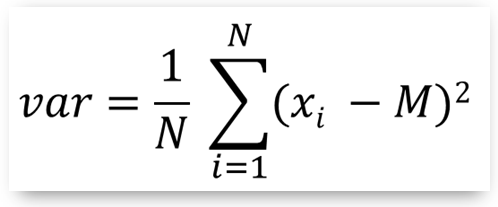
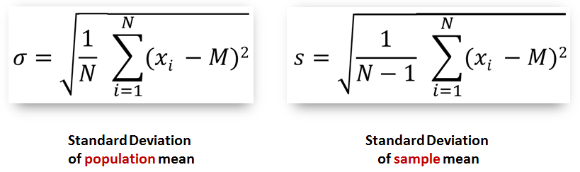
However, the standard deviation is the measure typically used in statistics to calculate and express the degree of dispersion of a set of data and it is defined as the square root of the variance:
standard deviation = sqrt(variance)The important thing you need to know about standard deviation, is: standard deviation of popoulation mean ('σ') is calculated slightly different from standard deviation of sample mean ('s') as you can see in the figure below.
- If you want to go deeper in standard deviation you can read more following the links bellow:
(C) Calculating your own standard deviation
- Standard deviation functions of the various statistical packages most often return the 'SD of sample mean' deviation ('s') dividing by N-1.
- However, the benfit of working with a real programming language is that we can build our own algorithm for computing standard deviation and divide by whatever we need. This is what we do in the following.
In [12]:
import numpy as np
import statistics as st
import pandas as pd


def mystd(dt, kind='sample'):       # kind: {sample, population, unbiased}
    # N: data size
    N = len(dt)
    #print(N)

    # M: mean
    M = dt.mean()
    #print(M)

    #SS: Sum of Squares
    SS = np.sum(pow((dt-M),2))
    #print(SS)

    #variance
    if kind == 'sample':
        var = SS/(N-1)
    elif kind == 'population':
        var = SS/N
    elif kind == 'unbiased':
        var = SS/(N-1.5)
    else:
        return 'kind should be {population, sample, unbiased}'

    return np.sqrt(var)

ar = np.array([1,2,3,4,5,6,7,8,9,10])
print(ar.std())
print(st.stdev(ar))
print(mystd(ar, kind='sample'))
As a practice
- In the above code we print three different 'std' values but only two of them are the same. Why?
- Check the documentation of numpy.std and statistics.stdev to deeper understand how the std functions work
- Furthermore: read the data from 'researchdata.csv' file and compute the standard deviation of the Control group data set (use the pandas DataFrame std method). Which type of standard deviation does this method compute? How can you change this?

Copyright
 . Free learning material
. See full copyright and disclaimer notice