Two way ANOVA (factorial)¶

In this section you will learn what is and when to apply the 'two way ANOVA' and again I will show you how to write and use a relevant function.

Understanding 'Two way' ANOVA¶

Two way ANOVA is the type of ANOVA control that we apply when we want to investigate the combined impact of two independent factors (variables) on one dependent variable that we measure.
To better understand the two way ANOVA see the table below where the columns represent the C levels that one independent factor may have, while rows represent the R levels of the other independent factor.

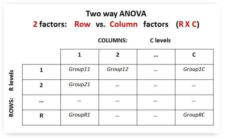
In the following we will use the 'RxC' notation to express the idea that we have a two way ANOVA with R rows (levels of 'Row' factor) and C columns (levels of 'Column' factor).

A two way ANOVA scenario¶

Continuing the 'background music' scenario: Suppose we suspect that the various music genres have a different impact on boys and girls. Thus, we introduce a new independent factor with two levels in our design (gender: 'M' (boys) or 'F' (girls)).
Now we have a '2 x 3' design of two way ANOVA, with a representation table that looks like this:

The two way ANOVA test will help us identify whether there are pair of groups in the above design for which the difference of the mean values is statistically significant.

The F statistic is once again computed starting from the general formula:

          MS between groups
  F = --------------------- 
          MS within groups

However, the nominator "MS between groups" needs now to be further analyzed in more than one components.
The key idea is that when we have two independent factors then the combined "between groups" variability is due to three distinct sources:
- (a) The impact of the 'Row' factor (MS_rows)
- (b) The impact of the 'Column' factor (MS_cols)
- (c) The impact due to the interaction of the two factors (MS_int)
Once again, we need to compute the above components and fill up the two way ANOVA table (see further below)

Reading resources¶

To better understand the two way ANOVA rationale you are encouraged to read the tutorial at 'Concepts & Applications of Inferential Statistics' which has provided also the basis for the ANOVA algorithm presented here.
I too provide more explanations as comments in the code below.

ptl_anova2(): a function for two way ANOVA¶

Below is the ptl_anova2() function for implementing two way ANOVA on input data.
Like before we are going to use some additional functions:
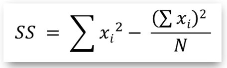
- ssd(): returns the sum of squared deviates for a series object containing the sample group data. Computed as:
- ssd_df(): as the ssd() above for a Series, the ssd_df() returns the sum of squared deviates for data in a DataFrame taken as a whole.
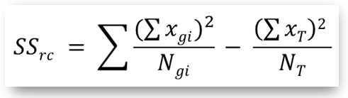
- ssd_df_rc(): returns the sum of squared deviates for specific groups in the anova table (either rows or columns). This sum is computed as:

where:

x_gi: data in the i-th group (in rows or columns depending on what we compute)

N_gi: the sample group size in the i-th group (in rows or columns)

x_T: data of the whole set of data

N_T: the number of all data (measurements)

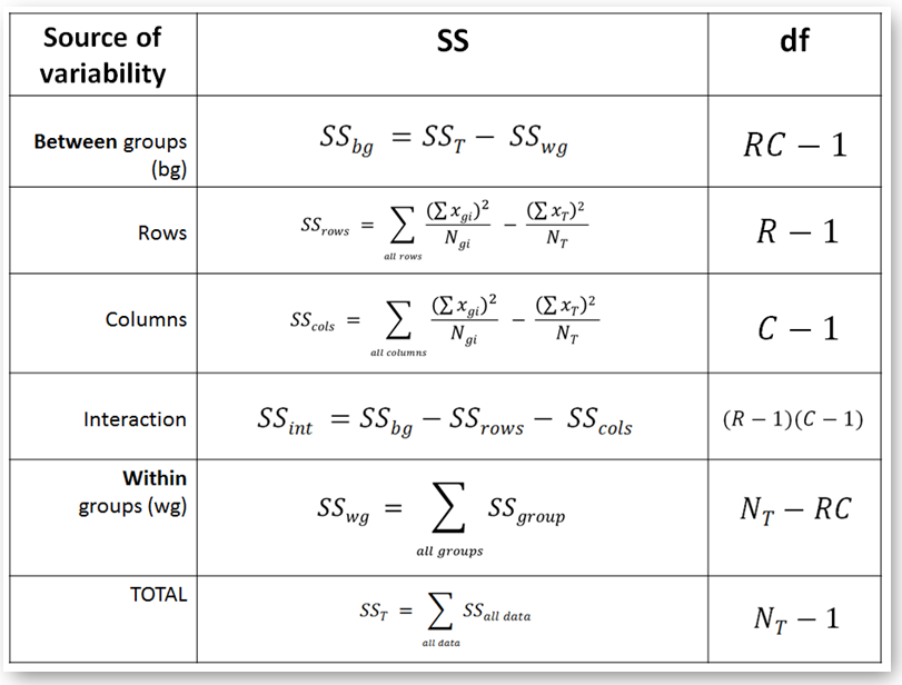
With the help of the above functions we are going to compute the quantities in the following 'two way anova' table

import numpy as np 
import pandas as pd
from scipy.stats import f

# import warnings
# warnings.filterwarnings("ignore", category=np.VisibleDeprecationWarning) 


def ssd(ser):
    '''
    Function ssd(): computes the sum of squared deviates for a Series object
    
    > Input parameters:
    - ser: the Series object
    
    > Returns:
    - The sum of squared deviates computed as Σ(x)**2 - ((Σx)**2)/N  
    '''
    ser.dropna(axis=0, inplace=True)     # Clear Series from null values 'in place'
    s1 = pow(ser,2).sum()
    s2 = pow(ser.sum(),2) / ser.size
    return s1-s2



def ssd_df(indf):
    '''
    Function ssd_df(): computes the ssd: Σ(x)**2 - ((Σx)**2)/N factor for a DataFrame object as a whole
      
    > Input parameters:
    - df: the DataFrame object
    It is ALWAYS assumed that the 1st column (0-index) is the R-factor and is ommited from computations
    
    > Returns a tuple consisting of:
    - ss_n_all = The ssd: Σ(x)**2 - ((Σx)**2)/N factor 
    - n_all = The size of DataFrame data included in the computation 
    '''
    
    n_all = sumx = sumx2 = 0
    for i in range(1,len(indf.columns)):
        ser = indf.iloc[:,i].dropna()
        sumx += ser.sum()
        sumx2 += pow(ser,2).sum()
        n_all += ser.size        
    sumx_sqed = pow(sumx,2)
    ss_n_all = sumx2 - (sumx_sqed / n_all)
    return ss_n_all, n_all



def ssd_df_rc(df, axis=0):
    '''
    Function ssd_df_rc(): computes the sum of squared deviates for the two way anova rows or columns  
    This sum is computed as Σ((Σ(x)**2)/Ν) - ((Σx_all)**2)/N_all
    It is ALWAYS assumed that the 1st column (0-index) is the R-factor and is ommited from computations
    
    > Input parameters:
    - df: the DataFrame object
    - axis=0 column-wise (working on columns data)
    - axis=1 row-wise (working on rows data) 
    
    > Returns:
    - The sum of squared deviates for the anova rows or columns of the input DataFrame
    '''
    
    ss_n_sum = 0
    ss_n_all = 0
    
    if axis == 0:
        # Compute the ss_n_sum quantity considering each SEPARATE Column in df 
        for i in range(1,len(df.columns)):
            c_ser = df.iloc[:,i].dropna()
            ss_n_sum += pow(c_ser.sum(),2) / c_ser.size
    
    elif axis == 1:
        r_factor = df.columns[0]
        anv_groups = df.groupby(r_factor)
        for symb, gp in anv_groups:
            # Compute the ss_n_sum quantity considerint each SEPARATE Row in df
            # Rows in df are ADDED columns in each anv_groups
            n_all = sumx = 0
            for i in range(1,len(gp.columns)):
                ser = gp.iloc[:,i].dropna()
                sumx += ser.sum()
                n_all += ser.size        
            ss_n_sum += pow(sumx,2) / n_all

    else:
        print('axis undefined in ssd_df_rc()')
        return 

    # Compute the ((Σx_all)**2)/N_all factor for ALL data in the DataFrame
    n_all = sumx = sumx_p2 = 0
    for i in range(1,len(df.columns)):
        ser = df.iloc[:,i].dropna()
        sumx += ser.sum()
        n_all += ser.size        
    sumx_sqed = pow(sumx,2)
    ss_n_all = sumx_sqed / n_all
    
    return ss_n_sum - ss_n_all
    


def ptl_anova2(inframe):                  
    '''
    Function:  ptl_anova2() for performing TWO way anova on input data
    
    > Input parameters:
    - inframe: pandas DataFrame with data groups as follows: 
    --- Column 0: the R-factor determining grouping
    --- Other Columns: Data grouped according to C-factor

    > Returns:
    - F: the F statistic for the input data
    - p: the p probability for statistical significance    
 
    '''
    # Detecting the shape of inframe:
    rows, cols = inframe.shape
    
    # Detecting the R x C anova design 
    c = len(inframe.columns)-1
    r_factor = inframe.columns[0]
    anv_groups = inframe.groupby(r_factor)
    r = len(anv_groups)

    # Computing ss_t and n_t with the ss_df() function
    ss_t, n_t = ssd_df(inframe)
    
    # Computing ss_wg with groupby.agg()
    ss_wg = 0
    ss_wg_cells = anv_groups.agg(ssd)
    ss_wg = ss_wg_cells.sum().sum()
     
    # Compute ss_bg by subtracking ss_wg from ss_t
    ss_bg = ss_t - ss_wg
       
    # ADDITIONAL (compared to One-way) computations in Two way ANOVA: ss_r, ss_c, ss_int
    # a) ss_c
    ss_c = ssd_df_rc(inframe, axis=0)
    
    # b) ss_r
    ss_r = ssd_df_rc(inframe, axis=1)
    
    # c) ss_int
    ss_int =  ss_bg - ss_r - ss_c 
      
    # degrees of freedom
    df_t = n_t - 1
    df_bg = r*c - 1
    df_wg = df_err = n_t - r*c
    df_r = r - 1 
    df_c = c - 1
    df_int = df_r * df_c
    
    # Mean Square (MS) factors
    ms_r = ss_r / df_r
    ms_c = ss_c / df_c
    ms_int = ss_int / df_int
    ms_wg = ms_err = ss_wg / df_wg
            
    # F, p
    F_r = ms_r / ms_err
    p_r = f.sf(F_r, df_r, df_err, loc=0, scale=1)
    
    F_c = ms_c / ms_err
    p_c = f.sf(F_c, df_c, df_err, loc=0, scale=1)
    
    F_int = ms_int / ms_err
    p_int = f.sf(F_int, df_int, df_err, loc=0, scale=1)
    
    # Printouts
    print('  bg: \t SS = {:9.3f}, \t df = {:3d}'.format(ss_bg, df_bg))
    print('Rows: \t SS = {:9.3f}, \t df = {:3d}, \t ms = {:9.3f}, \t F = {:9.3f}, \t p = {:8.4f}'\
          .format(ss_r, df_r, ms_r, F_r, p_r))
    print('Cols: \t SS = {:9.3f}, \t df = {:3d}, \t ms = {:9.3f}, \t F = {:9.3f}, \t p = {:8.4f}'\
          .format(ss_c, df_c, ms_c, F_c, p_c))
    print(' Int: \t SS = {:9.3f}, \t df = {:3d}, \t ms = {:9.3f}, \t F = {:9.3f}, \t p = {:8.4f}'\
          .format(ss_int, df_int, ms_int, F_int, p_int))      
    print('  wg: \t SS = {:9.3f}, \t df = {:3d}, \t ms = {:9.3f}'.format(ss_wg, df_wg, ms_wg))
    print('TOTL: \t SS = {:9.3f}, \t df = {:3d}'.format(ss_t, df_t))
    
    
    return


# Main ========================================================================

# Pre-set data for repeated measures TWO way ANOVA validation
# These data are copied from http://vassarstats.net/textbook/index.html
# testdata = pd.read_excel('../../data/researchdata.xlsx', sheetname="anova2test")

# ALTERNATIVE: Read data from file 
testdata = pd.read_excel('../../data/researchdata.xlsx', sheetname="anova3x2")

ptl_anova2(pd.DataFrame(testdata))

  bg: 	 SS =    38.317, 	 df =   5
Rows: 	 SS =     1.789, 	 df =   1, 	 ms =     1.789, 	 F =     1.021, 	 p =   0.3155
Cols: 	 SS =    35.927, 	 df =   2, 	 ms =    17.963, 	 F =    10.249, 	 p =   0.0001
 Int: 	 SS =     0.601, 	 df =   2, 	 ms =     0.301, 	 F =     0.171, 	 p =   0.8427
  wg: 	 SS =   138.460, 	 df =  79, 	 ms =     1.753
TOTL: 	 SS =   176.776, 	 df =  84

Interpretation of results¶

As you see in two way ANCOVA we calculate three F ratios: F_rows, F_columns and F_interactions and each one of them tells its own story.
F_rows and p_rows provides information about the R-factor. In our example p_rows is well above the 0.05 threshold and therefore the R-factor ('Gender') does not seem to have any impact on the outcome: boys and girls are likewise affected by the different mosice genres.
Contrastingly, F_columns is big enough to make p_columns extremely low. Therefore, we identify a main effect: the C-factor (the various conditions of treatment) has a significant impact on student learning.
Finally, F_interaction appears to be extremely low with a high p_interaction meaning that the combined effect of R-C factors is insignificant.

Remember that ANOVAs only return a valuable information for understanding whether significant differences exist between the group means when investigating the variances of the groups taken as a whole.
You need to additiionally apply Tukey's HSD test (as demonstrated in the one way ANOVA section) to identify the group or groups that are responsible for this difference.

Download¶

Download the ptl_anova2() code as .py file

Copyright¶

. Free learning material
. See full copyright and disclaimer notice