Write your own ANOVA function¶

Why?¶

In this section I will show you how to write your own ANOVA function. But why should one want to do this? (apart, of course, from engaging in a good code skill development form of practice).
In my opinion, these are some reasons:
- (a) Code developed by others does not always return the results you would like to have; for example, scipy anova method f_oneway() does not return any effect size (and this holds true for commecrial statistical packages as well). It would be nice to be able to write a few lines of code and improve the quality of your work and reported results.
- (b) Scipy currently does not support more advanced forms of ANOVA analysis (ANCOVAs, MANOVAs, etc.). Other packages (like 'statsmodels') do support this form of analysis up to a certain point but in a rather complex way compared to the solution presented here. Remember also that writing your own functions not only gets you further beyond but makes you a potential contributor to the Python/Scipy community.
- (c) Writing your own statistical functions helps you better undesrtand statisticis and that makes you a better qualified researcher.
Understandably, writing code is more demanding than using ready made modules. However, it seems to me that if you have successfully made your way up to this point of the pytolearn tutorials it won't hurt much to follow through "writing your own ANOVA". Once successful in this task you can always explain to your fellow researchers -who might ask you about the statistical package you are using- that "I am writing my own code!" (retaining, of course, an appropriately humble voice tone ;-)

Understanding ANOVA¶

You have to understand the ANOVA 'way of thinking' before writing your code and this is what we are going to do first. Note also, that at the end of this section I will provide some relevant resources and other directions that you could possibly follow. So, what is ANOVA?

ANOVA is a statistical control investigating the null hypothesis that the mean values of k samples (M_i) are statistically not different from each other.

H₀: M₁ = M₂ = ... = M_k

The alternative H_a is , of course, that there exists at least one pair of samples with statistically different mean values.

To test the above hypothesis ANOVA follows the general noise/signal pattern and computes the F statistic based on the following formula:

Thus, the ANOVA line of thinking postulates that there will always be some kind of "unexplained" variability (due to uncontrolled factors) in measurements of the dependent variable within groups (the 'noise' in the above equation), AND there will also be some "explained" variability (due to the examined controlled factor) when comparing measurements between groups (the signal) .
What we want to know is whether the signal is strong enough so that the probability of measuring such a large F value is really small (smaller than the 'a' threshold level). If this is the case, then we accept that the difference between the mean values in at least one group pair is statistically significant.

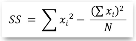
Remember now that for a set of measurements (sample) the variability is calculated as the sum of squared deviates from the mean value of the sample: 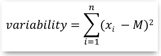where:
- n: sample size
- x_i: data in the sample (single measurements)
- M: the sample mean

Based on this idea, we compute transform the nominator and denominator of the F ratio as follows:
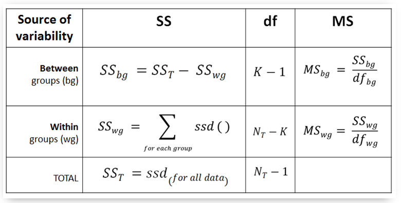
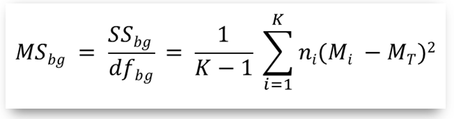
- Nominator: As between group variability we take the mean square between group quantity (ms_bg), computed by:
where:
- SS_bg: the sum of squared deviates from the total mean value M_T
- df_bg: the degrees of freedom "between groups" (equal to K-1)
- K: number of samples (groups)
- n_i: number of data (measurements) in the i-th sample (group)
- M_i: the mean value of the i-th sample
- M_T: the total mean (considering the data in all samples)

Respectively, as within-group variability we take the mean square within group quantity (ms_wg), computed by:

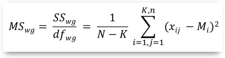
where:

SS_wg: the sum of squared deviates from each sample mean value M_i

df_bg: the degrees of freedom "within groups" (equal to N-K)

N: the overall sample size (n₁ + n₂ + ... + n_k)

x_ij: data in the sample groups (single measurements), the j-th measurement in the i-th (out of k) groups

M_i: the mean of the i-th (out of k) sample (group)

Therefore, to compute F we need to compute the above ratio of MS_bg / MS_wg

Please note:¶

The above is but a concise introduction to the ANOVA rationale. If you are interested in more details you may read an extended "Conceptual Introduction to the Analysis of Variance", which has provided the theoretical basis for the computational process of implementing ANOVA, that is presented in this and the following tutorials.
In some tutorials the terms 'effect' and 'error' are used to identify the nominator and denominator quantities. Indeed, in one way ANOVA 'effect' and 'error' are identical to 'between groups' and 'within groups' variability respectively. However, these latter terms are more general and -as you will read in next sections- can be analyzed to include more variability factors than 'effect' and 'error'.

ptl_anova1(): a function for one way ANOVA¶

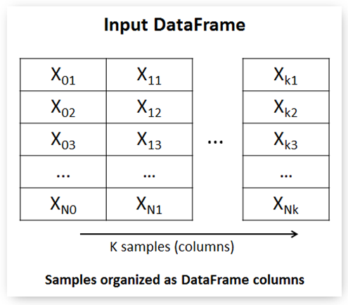
Below is the ptl_anova1() function ('ptl' prefix = 'pytolearn') for applying 'one way anova' on data in a DataFrame. Each sample group is a column in the input DataFrame.
There are two other functions useful in ANOVA computations (we will use them in next sections as well), namely:
- ssd(): returns the sum of squared deviates for a series object containing the sample group data. To compute SS the function makes use of the formula: which is algebraically equivalent to the above formulae for MSbg and MSwg.
- dftoser(): converts a DataFrame to a Series object; useful to compute the ssd() for the whole DataFrame data.

With the help of the ssd() function we are going to compute the quantities in the following anova table

The function docstrings provide initial documentation regarding function input and output.
Note the 'vectorized' operations which make obsolete the use of loops in many situations (for example, when calling pow() for the ser object to compute the squares in the ssd() function)
The function prints out many outcomes much like a statistical software package would do. However, the advantage of working with open code is that you can modify and enrich these outcomes anyway you like.
To compute the probability p the function makes use of the sf() function which is available from the imported scipy.stats.f module. If you are unfamiliar with the use of this (and other similar) functions you may wish to read the relevant section on 'Distributions'

import numpy as np 
import pandas as pd
from scipy.stats import f


def ssd(ser):
    '''
    Function ssd(): computes the sum of squared deviates for a Series object
    
    > Input parameters:
    - ser: the Series object
    
    > Returns:
    - The sum of squared deviates computed as Σ(x)**2 - ((Σx)**2)/N  
    '''
    ser.dropna(axis=0, inplace=True)     # Clear Series from null values 'in place'
    s1 = pow(ser,2).sum()
    s2 = pow(ser.sum(),2) / ser.size
    return s1-s2


def dftoser(df):
    '''
    Function dftoser(): converts a DataFrame to a Series appending all columns in place
    
    > Input parameters:
    - df: the DataFrame object to be converted
    
    > Returns:
    - A Series object containing all DataFrame columns one after another    
    '''
    # Clear DataFrame from null values 'in place' and possibly drop 'all NaN' rows or columns
    df.dropna(axis=(0,1),how='all',inplace=True)   
    
    ser = pd.Series()
    for i in range(len(df.columns)):
        ser = ser.append(df.iloc[:,i])
    return ser


def ptl_anova1(inframe):                  
    '''
    Function:  ptl_anova1() for performing 'one way anova' on input data
    
    > Input parameters:
    - inframe: pandas DataFrame with sample groups in columns (one column for each group)
    
    > Returns:
    - F: the F statistic for the input data
    - p: the p probability for statistical significance
    '''
    
    # Number of sample groups
    k = len(inframe.columns)
    
    # Convert dataframe to a series object
    allser = dftoser(inframe)
    n_t = allser.size
    
    # degrees of freedom
    df_t = n_t - 1
    df_bg = k - 1
    df_wg = n_t - k
    
    # Compute ss_t (total)
    ss_t = ssd(allser)

    # Compute ss_wg as sum of ss for all samples ( = columns in the 'inframe' DataFrame)
    ss_wg = 0
    for i in range(k):
        ss_wg += ssd(inframe.iloc[:,i])
    
    # Compute ss_bg by subtracking ss_wg from ss_t
    ss_bg = ss_t - ss_wg
    
    # Mean square within groups  ('error')
    ms_wg = ss_wg / df_wg
    
    # Mean square between groups  ('effect')
    ms_bg = ss_bg / df_bg
    
    
    # Compute F, p
    F = ms_bg / ms_wg 
    p = f.sf(F, df_bg, df_wg, loc=0, scale=1)
    
    # Printouts
    print('Between groups (effect):\t SS_bg = {:8.4f}, \t df_bg = {:3d}, \t ms_bg = {:8.4f}'.format(ss_bg, df_bg, ms_bg))
    print('  Within groups (error):\t SS_wg = {:8.4f}, \t df_wg = {:3d}, \t ms_wg = {:8.4f}'.format(ss_wg, df_wg, ms_wg))
    print('                  TOTAL:\t  SS_t = {:8.4f}, \t  df_t = {:3d}'.format(ss_t, df_t))
    print('F = {:8.4f}, p = {:8.4f}'.format(F, p))        
    
    return F, p


# Main ========================================================================

# ALTERNATIVE-1: Pre-set data for validating the 'one way ANOVA' code
# These data are copied from http://vassarstats.net/textbook/index.html
# testdata = {'G0':[27.0, 26.2, 28.8, 33.5, 28.8],
#             'G1':[22.8, 23.1, 27.7, 27.6, 24.0],
#             'G2':[21.9, 23.4, 20.1, 27.8, 19.3],
#             'G3':[23.5, 19.6, 23.7, 20.8, 23.9]
#            } 



#=============================================================================
# ALTERNATIVE-2: Generate randomized data for testing 
# testdata = {'G1':[np.random.randint(1,101) for i in range(100)],
#             'G2':[np.random.randint(1,101) for i in range(100)],
#             'G3':[np.random.randint(1,101) for i in range(100)]
#             }

#=============================================================================
# ALTERNATIVE-3: Read data from file 
testdata = pd.read_excel('../../data/researchdata.xlsx', sheetname="anova")

F, p = ptl_anova1(pd.DataFrame(testdata))

Between groups (effect):	 SS_bg = 1115.9100, 	 df_bg =   2, 	 ms_bg = 557.9550
  Within groups (error):	 SS_wg = 14583.4020, 	 df_wg = 126, 	 ms_wg = 115.7413
                  TOTAL:	  SS_t = 15699.3120, 	  df_t = 128
F =   4.8207, p =   0.0096

A last comment¶

We have seen now much clearer the inner mechnics of ANOVA. Hopefully, it is understandable how the "signal/noise" ratio has been gradually transformed to a computatable representation of an F variable distribution.
In the next tutorials on the ANOVA family we will also follow a similar approach, explaining how the "between groups" and "within gropus" variability should be interpreted.

Practice: compute effect sizes¶

Formulae for effect sizes (eta squared and omega squared) are available here (by 'The Analysis Factor').
As a practice write the code so that the ptl_anova1() prints out both eta and omega squared effect sizes.

Download¶

Download the ptl_anova1() code as .py file

Copyright¶

. Free learning material
. See full copyright and disclaimer notice